Problem 1 - b
Given conditions: \(U\) = 1, \(\Gamma\) = 0.1, and \(Q\) = 0. Use TDMA to find \(\phi\).
- Plot \(\phi\) vs. \(x\) on the same graph using grid sizes of \(N\) = 10, 20, 30, 40, 50 and compare your result to the analytical solution.
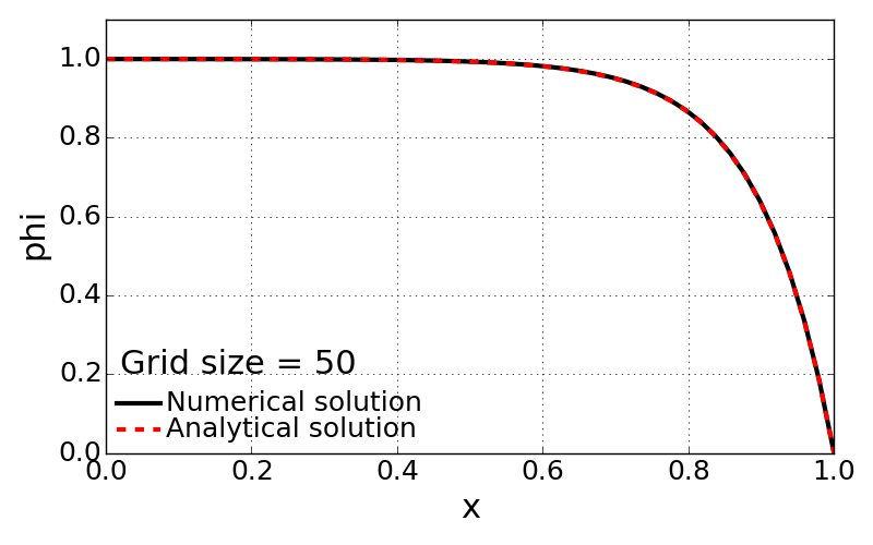
- Grid size, N = 50 with full scale
- Discussions on numerical solution
- As observed in the first figure, the final solution looks having strong convection effect with such a flat upstream solution and getting (diffused) down to the boundary fixed value at right wall.
- The numerical solution with 50 grid points is having consistent match with exact solution.
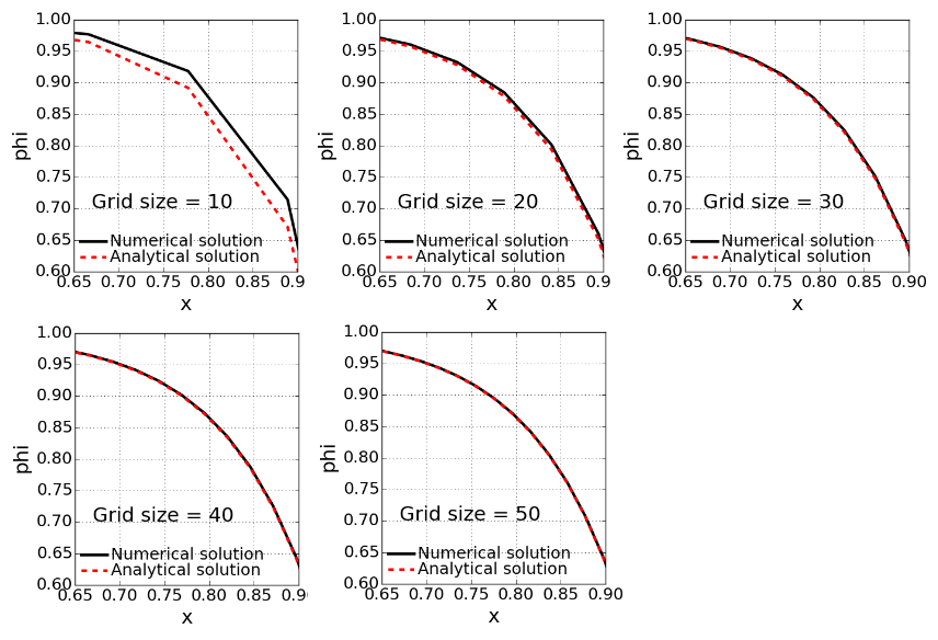
- Effect of grid size on numerical solution in magnified scale
- Discussions on grid size effect
- Deviation of numerical simulation from the analytic solution is getting bigger as the grid become coarser.
- Biggest inaccuracy in numerical solution (descretization errors) with the case of \(N\) = 10.
- Plot the average error as a function of \(N\) in a log scale and normalization with respect to grid size.
Here the average error is defined as Root Mean Square of deviation of numerical solution from the analytical solution. The calculation was done with the following definition.
\[err = \frac{\sqrt{\sum_{i=1}^{N}(\phi_i - \phi^{exac}_i)^2}}{N}\]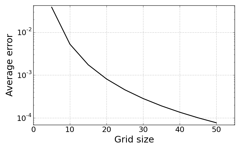
- Discussion
- Here, the average error is dropping dramatically as the smaller grid size is used.
- As the central descritization is applied for finite difference, the accuracy is improved with second order accuracy.
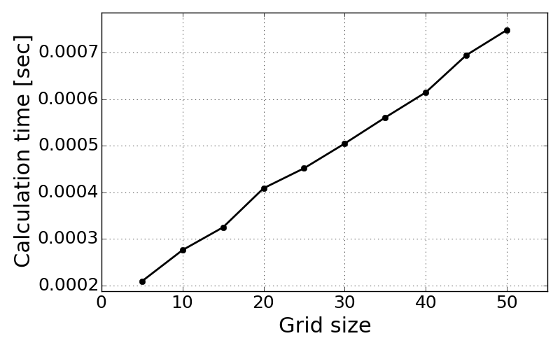
- Examine how the calculation time changes with \(N\) and evaluate the time complexity of the algorithm.
The computational time is defined as the consumed real calculation time while the numerical solution is being solved. The time is measured only during the numerical scheme process, meaning that pre-processing and post-processing time has been eliminated.
- Discussion
- The compute time is increased linearly as the grid size become bigger.
- The linear increment of time is because of the 1-dimensional grid use.
- The currently used solver, TDMA sweeps back and forth one time along the grid points to have solutions of system of linear equations. Thus, the actually calculation time must be only dependent on the number of node points.