Problem 2 - g

Solve the problem using a 2-level geometric multigrid method. Compare the computational time with other methods.

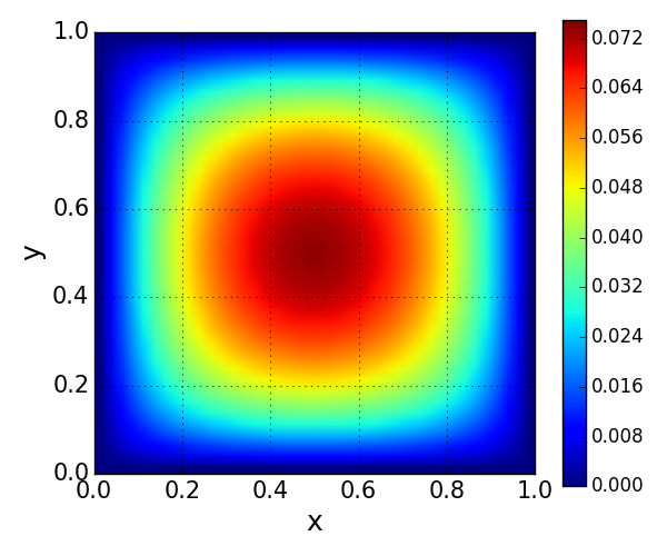
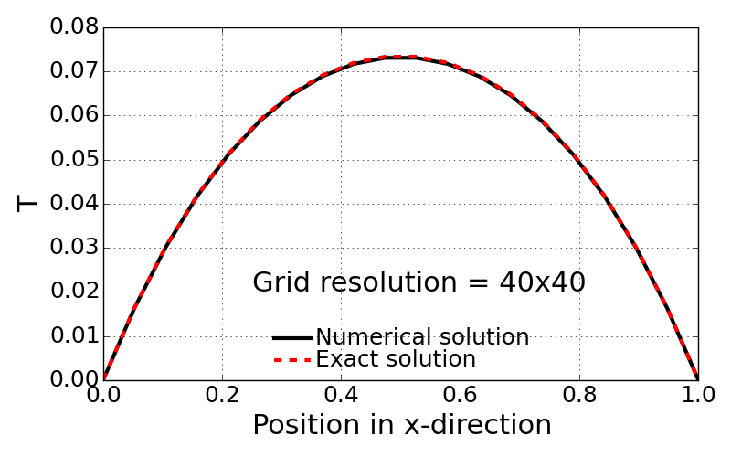
Following figures show the contour and line plots of multigrid solution with Gauss-Seidel method. Those two figures are illustrating converged temperature solution consistent with the previous solution obtained by the other methods.

The following tests were performed on 40x40 grid case. Four different setup has been set to find the performace of multi-grid method.

test case	Main-iteration # at final	Computation time
Jacobi w/o MG	2069	42.83 sec
Jacobi w/ MG	20	14.07 sec
G-S w/o MG	1035	27.49 sec
G-S w/ MG (1)	8	13.28 sec
G-S w/ MG (2)	14	13.78 sec

• Discussions
  • The multi-grid has been tested on different set of numerical methods and different sub-iteration numbers. The best solution was achieved by using 10 sub-iteration on coarse grid with properly specified \(e\) matrix.
  • The computational time with multi-grid method was reduced by a factor of 2 for G-S and 3 for Jacobi.
  • Interestingly, using multi-grid method and its fast convergence cover up the slowness of Jacobi method: Note the computational time between G-S and Jacobi is not significant when multi-grid is used.

• Effect of initial condition for \(e\) matrix on coarse grid.
  • The final two test cases with G-S with multi-grid were conducted with the different initial condition for \(e\) matrix on coarse grid.
  • The first one ‘G-S w/ MG (1)’ runs with non-zero value of initial condition for \(e\) matrix. The initial condition was set from the half of errors between current time level solution and exact solution.
  • The reason that ‘half’ of the error was used is to avoid the divergence. Under relaxing effect in initial condition was helpful to improve the convergency in coarse grid.
  • On the other hand, the zero set of initial condition for \(e\) matrix required more iterations. But total computational time is not significantly far away from the first test case, ‘G-S w/ MG (1)’.